Portfolio Construction Theory: Risk

This article will cover some of the major principles and topics when constructing a portfolio of securities. The focus is risk management.

Article will cover:

1. Risk terminology
2. The rebalancing aspect of a portfolio
3. The weighting by beta
4. The concepts of variance, covariance and correlation
5. The calculation of the portfolio variance, St. Deviation
6. Value at Risk

Risk

I will define risk as losing money. Big risk -> lots of money can be lost. Small risk -> a safe amount of money can be lost.

Money can be lost when buying or selling a position & then price moving avertedly due to a variety of factors. Horrible psychology, leading to awful decisions, a meteorite crashing into a major city, Earthquake in New York or the inflation going out of hand. Some are more likely than other.

When buying a position in a single stock, the stock has two types of risk. Systematic and.. Unsystematic. In an unlikely situation of a major earthquake happening in NYC, the overall stock market could go down quite a bit. This would push the stocks’ price down and it is called a systematic risk. It is not due to the stock underperforming, rather the market itself. Unsystematic risk is the contrary. The CEO of the company spending all of its money on a huge yacht, sex scandal or simply bad earnings- this would lead to a depreciating price for the single stock, not the market itself.

And then lastly we have a risk of horrible decision making. In Lithuania we have a saying “the is no medicine from stupidity”, so this risk is for another article. I’m afraid it would take too much space trying to figure it out.

Coming back to the financial risks, it is natural that we want to decrease the risk. However, we will find ourselves balancing between systematic and unsystematic risks. Unsystematic risk while being the larger, usually brings more returns, hence we wouldn’t want to get away from it completely. The ideal situation, we are to find, is having several stocks, thus increasing the systematic risk, however decreasing unsystematic as much as we possibly can in order to optimize our risk/reward ratio. (meaning trying to keep returns high but demolish risk).

Rebalancing

Imagine you buy TSLA stock. TSLA rises by $1: you have earned one dollar! Now add a AAPL short. If AAPL rises by $1 and TSLA rises by $1, the current profit is 0, however if AAPL would rise by $0.5, then our profit would be $0.5, offset by the TSLA . This is simple.

If we hold this position for a while, it is highly likely that the prices of these assets will differ by a larger and a larger amount. In this case, if we had that position from 2022 to 2023, the TSLA would have outperformed the AAPL by a large amount and so it would take up more “space” in the portfolio. A simple example: If TSLA rose from $1 to $5 and AAPL rose from $1 to $1.5, then the overall portfolio value is: $5 + $0.5 (AAPL short lost 50% of value), therefore we now have 90% of TSLA stock and only 10% of AAPL.

Rebalancing means that we equal out both positions (in this case sell TSLA and add AAPL short) until they are equally sized. Ideally, rebalancing should occur as frequently as possible, however trading fees, time consumed, and the bid-ask spread would start eating out the profits rapidly, if rebalancing is too often, therefore there is a tradeoff between the frequency (and so efficiency of the portfolio) of rebalancing and the trading fees.

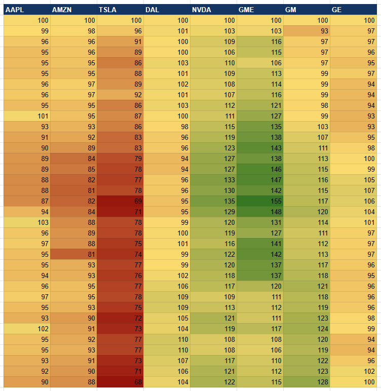
Below (Fig. 2) is the returns chart of this position when non-rebalanced, rebalanced every 2 weeks and rebalanced every day.

As you can see, the Non rebalanced portfolio has the largest peak, however it also had the largest drawdown, when compared the rebalanced portfolios. Portfolio that has been rebalanced periodically has shown superior returns. The reason is that big market moves take time to appear. If given a period of 2 weeks, portfolio still captures the short-term growth before dropping some position and equalizing the portfolio.

As suspected, the TSLA has the largest share of the portfolio at the time of the drawdown, see Fig. 3 below.

To prevent this, simply rebalance every two weeks. The weights chart is shown below (Fig. 4). On average, the weights will be almost equal on a larger period of time.

Beta Weighting

Beta shows how much more an asset moves when compared to the market. 1 is exactly the same, 2 is twice of that. (If market grows by 1%, then asset with a beta of 2 is expected to grow by 2%. Beta -1? Then asset is expected to fall by 1%)

Let’s call beta our risk. The larger beta stocks we own, the more risk our portfolio has. The key is to level out all positions so they offer the same amount of risk. Let’s set an example:

TSLA Beta: 2.26 | AAPL Beta: 1.3

To level the position out, we should have twice the AAPL than TSLA. A formula to calculate it is: 1. Average all betas of the portfolio. 2. Divide the current beta by the portfolio Beta 3. Result is the percentage of how much we need to adjust the portfolio.

See the spreadsheet below. Let’s assign an equal weight to some stocks. Let’s fetch their Beta’s and then calculate how much do we need to adjust the weights so that the risk is similar to all of our positions.

Ticker	AAPL	AMZN	TSLA	DAL	NVDA	GME	GM	GE
Weight	12.50%	12.50%	12.50%	12.50%	12.50%	12.50%	12.50%	12.50%
Beta	1.3	1.17	2.26	1.39	1.69	-0.26	1.48	1.29
Weight Adjustment to Neutral	99.23%	110.26%	57.08%	92.81%	76.33%	496.15%	87.16%	100.00%

The Adjusted Weights of each position will be “Weight Adjustment to Neutral” divided by “Weight” from the Table 1.

Let’s sum them all up. The result is around 140%. But we started with 100% as our original weights! Further adjustment needed. For that, simply divide the “Adjusted Weights” by “Total”.

Adjusted Weights	12.40%	13.78%	7.13%	11.60%	9.54%	62.02%	10.90%	12.50%
Total	139.88%
Final Adjusted Weights	8.87%	9.85%	5.10%	8.29%	6.82%	44.34%	7.79%	8.94%

Lastly, we can construct the same rebalancing algorithm as for the AAPL-TSLA spread trade, but with all these tickers. As explaining here in the blog would be a rather difficult and not the most appealing thing, I am attaching the .xlsx file for your review. The orange cells are the ones to change. Model supports 8 positions, both long and short & constructs a historical backtest.

Variance & Covariance

Variance, in the context of stock prices, measures how much a stocks return varies with respect to its average daily (or any period used in calculation) returns. Formula is very simple.

Where:

X = Return
µ = Average return
N = Total number of returns

The square root of variance is standard deviation- one of the most common risk measures.

Covariance, in the context of stock prices, indicates how the variables move together. It tells us whether variables move to the same direction, or the opposite. The covariance, however, does not tell us about the magnitude. It’s the job of correlation (I suppose the reader understands the concept of a correlation). See the formula below.

Where:

Rt S1 = Return of stock 1
Avg Rt S1 = Average return of stock 1
Rt S2 = Return of stock 2
Avg Rt S2 = Average return of stock 2

Variance Covariance Matrix

This is one matrix. If there are 10 securities in the portfolio, then this matrix will have the information for the variance of a stock, and it should also show the covariance between one security and the other 9. The same for each security.

However, the variance covariance matrix isn’t that much of a use. What we want is the correlation matrix, which would allow us to calculate the portfolio variance and thus, the portfolio standard deviation. This will give us a good approximation for the probabilities of the portfolio incurring certain losses, Value at Risk.

Imagine the portfolio of 5 stocks. The size of the matrix would be 5×5. The formula to create a variance covariance matrix is as follows.

Where:

k = No. of Stocks in the portfolio
n = No. of observations (returns)
X = n x k excess return matrix
X^T = Transpose matrix of X

The first step is to calculate the excess return matrix. This is split into two steps. First- get the data, calculate daily returns and then their average.

Secondly, compare each return to its average.

And that’s the X matrix from our formula.

The next step is transposing the excess returns matrix and then multiplying it by itself. This is done by a simple excel formula, where N6:R16 is the Excess returns matrix.

Last step is dividing the X^T*X matrix from n.

Correlation Matrix

Let’s kick it off by the formula of correlation.

Where:

Cov (x,y) = the covariance between 2 stocks
qx = St. Deviation of stock x
qy = St. Deviation of stock y

Because there is 5 stocks in our portfolio, we have to resort to the matrix multiplication. This one is going to be a ride, get a seat belt on.

First, get the standard deviations of each stock. Excel has a formula =STDEV()

Now we need to get the denominator. If we had only a couple of stocks, then this is quite easy, however when having 5 different ones, we have to have the product of all the standard deviations between all combinations of the stocks in the portfolio. To achieve this, multiply all a=standard deviations from themselves, but transpose first. (see fig 10)

After this is done, we divide each variance covariance from each standard deviation using (again) matrix multiplication, to get the correlation matrix.

This matrix gives us the corresponding correlation between every stock. Notice, however that this is a mirrored matrix, where each X security * X security is 1 and on the other side is a mirror image.

Note: I am aware that I had made a mistake in the GOOGL vs AAPL data: I used the same data, meaning their correlation is the same. However, I will leave the mistake as it is quite harmless in this example and I would need to change lots of pictures.

Portfolio Variance

Let’s begin with a formula.

Portfolio Variance = Sqrt (Transpose (Wt.SD) * Correlation Matrix * Wt. SD)

Remember, in the beginning of the article we were discussing the weightings of the stock in the portfolio. Well, it is time to get back to it. Once we assign weights, let’s multiply the standard deviation by its weight to get the weighted standard deviation. See fig 12.

Note, that since I didn’t use GOOGL in my original weightings part, I simply assigned a lot of weight to it so the total is a 100%.

Next step is to calculate the product of the Transpose of w. st. Deviations and call it a G1.

Now we multiply G1 by the weighted st. deviations. (Fig 14)

And for the last step-> square root of it to get the variance

The variance is 0.91% ! Phew! That’s a process.

Value at Risk (VaR)

Value at Risk (VaR) has been called the “new science of risk management,” and is a statistic that is used to predict the greatest possible losses over a specific time frame.

Commonly used by financial firms and commercial banks in investment analysis, VaR can determine the extent and probabilities of potential losses in portfolios. Risk managers use VaR to measure and control the level of risk exposure.

Once we have the portfolio variance, we simply take the square root out of it to get the standard deviation of the portfolio. In our case- 9.52% is the answer. What does it tell us?

The standard deviation assumes that the data is normally distributed and if so, we get our probabilities. See fig. 16

What this tells us is that there is 96% chance of staying within +-2 SD bound. Meaning there is 4% of going out. As we do not care (except for joy) about going out of bounds to the positive direction, there is a 2% chance of going below 2 Standard deviations.

Using 9.52%, we calculate that there is a 2% chance, that by having a portfolio variance of 0.91%, we our portfolio will go below 19.04%.

The downside of this? We know that the stock market does not exhibit a normally distributed curve and that the tail events happen much more frequently, thus a simple correction would be to give it a 4% chance, rather than 2%. This simply gives our approximation more “room to breathe”.

The better method is a Monte Carlo simulation, where we would use a jump diffusion process to model the market and get a more reliable bell curve, that has fatter tails. I cover this method in my previous articles.

Find the sheet with the portfolio variance and standard deviation below: